


Adolfo Crespo Márquez (1), Samir Shariff (2)

- Department of Industrial Management, School of Engineering, University of Seville, Seville, Spain.
- Department o Electrical engineering, Taibah University. Saudi Arabia
Abstract #
An Asset Health Index (AHI) is a tool that processes data about asset’s condition. That index is intended to explore if alterations can be generated in the health of the asset along its life cycle. These data can be obtained during the asset’s operation, but they can also come from other information sources such as geographical information systems, supplier’s reliability records, relevant external agent´s records, etc. The tool (AHI) provides an objective point of view in order to justify, for instance, the extension of an asset useful life, or in order to identify which assets from a fleet are candidates for an early replacement as a consequence of a premature aging.
Keywords: Assets management, capital investment, operation and maintenance decision making, life cycle analysis, assets health.
Introduction #
An Asset Health Index (AHI) is an asset score, which is designed, in some way, to reflect or characterize the asset’s condition and thus, its performance in terms of fulfilling the role established by the organization.
AHI represent a practical method to quantify the general health of a complex asset. Most of these as-sets are composed of multiple subsystems, and each subsystem can be characterized by multiple modes of degradation and failure. In some cases, it may be considered that an asset has reached the end of its useful life, when several subsystems have reached a state of deterioration that prevents the continuity of service required by the business.
Therefore, the health index, based on the results of operational observations, field inspections and laboratory tests, produces a single objective and quantitative indicator. It may be used as a tool to manage as-sets, to identify capital investment needs and maintenance programs, allowing:
Compare the health of equipment located in similar technical locations, to study possible premature deterioration and optimize operation plans and/or asset maintenance if necessary;
Communicate more accurately with manufacturers, understand the behaviour of assets of different manufacturers in specific technical locations;
Support decision-making processes in future investments in assets, or in extension of the life of these. Methodology.
The methodology requires an important number of input data to the index calculation models, such as the ones mentioned below:
The identification of the asset, which includes the category of the equipment under study, the current age, the expected life, the name of the manufacturer, the model of the equipment and the location of the installation.
The operation data recorded during a certain period of time, which combined conveniently allows us to know the time that the equipment has been working on stress, number of starts and stops, consumption, etc.
The condition of the equipment, that is, the results of the analyses performed on the equipment in site, results of readings of physical variables such as temperature and vibrations, results of visual inspections, thickness measurements, thermography, etc.
Development.
The application procedure for calculating the health index is based on 5 consecutive steps, in which, starting from an estimated normal life associated with an equipment’s category, a current health index is reached. For this, a series of factors related to the location, operation and condition of the asset are considered.
It is presented in the following Figure 1, the model, with the 5 steps for calculating the health index of an asset.
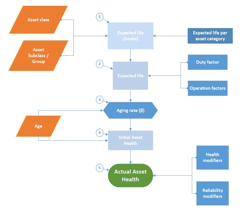
Figure 2. Procedure to calculate the AHI.
Step 1. Asset’s selection, definition of category and sub-category. Capture of UT data, physical asset, and obtaining the estimated normal life of the asset.
In this first step, the identification of the asset and all the information related to the functional location, such as:
Functional location of the location in the plant management system where the equipment is located.
Inside / outside situation of the asset. This parameter will be considered to determine the exposure to external agents that may affect the health of the asset.
The distance to the coast. This parameter will be taken into account, like the previous one, to know the possibility that the humidity and the corrosive environment due to being close to the coast, may cause damage to the health of the asset.
Average outside temperature. It is understood by the average of the exterior temperature, at the average annual temperature registered in the site and that can directly affect the performance of the equipment located there.
Exposure to agents such as: dust in suspension and corrosive atmosphere. The proximity of the facilities to industrial emission sources of dust in suspension and corrosive agents, can cause the acceleration of equipment deterioration in the long term.
Regarding the equipment information, we identify manufacturing data, model and technical design specifications for the preparation of tables that will be used later in the definition of health modifying parameters.
The estimated normal life of the asset is a data that, in general, comes from the technical direction of the company, considering the experience accumulated so far and the information provided by the different manufacturers.
The value of the estimated normal life is used as a starting point for the realization of all the calculations that will be seen below. Keep in mind that its value is approximate and only depends on the asset category. As we will see below, it will be modified by the characteristics of the location and loading.
Step 2. Impact’s evaluation of load and location factors by type of asset, technical location and estimated life expectancy.
Compiled all the information in the previous point, we proceed to the evaluation of the location and load factors (unambiguously associated with the technical location of the asset, as discussed previously). Since there is more than one variable that affects each one of the factors, for each of them a single combined factor must be calculated. Next, its obtaining is shown.
Depending on whether the asset is inside or outside a compartment that protects it from external agents, there are two ways to estimate it. If the technical location of the asset is external, the calculation of the combined factor of location is calculated following the equation shown below.
FE: Combined location factor.
FDC: Distance to the coast factor.
FA: Altitude above sea level factor.
FT: Annual average of outside temperature.
FAT: exposure to corrosive atmosphere factor.
FPS: exposure to dust in suspension factor.
In this case, being an element on the outside there is some factor greater than one (Fi ≥ 1), being Fi any of the factors contemplated above:
= max (FDC, FA, FT, FAT, FPS)
The load factor (FC), as well as the location factor, is inherent in the technical location. This factor measures the load request that is made on the equipment in that location, in front of the maximum admissible load. Normally, this data is obtained from the start-up and delivery of the equipment by the manufacturer, being recorded in the technical specifications of the equipment. In general, the following equation is used:
The Estimated Life of the asset is the quotient that results from dividing the estimated normal life obtained in the previous section, between the product of the location and load factors.
Therefore, depending on where the asset is located, and its expected level of performance, its useful life can be modified.
Step 3. Calculation of the aging rate.
A fundamental hypothesis of the chosen methodology is that the aging of an asset has an exponential behaviour with respect to its age. The aging rate is the parameter of the model that allows us to express mathematically this mode of behaviour, and take into account the different phenomena that the asset can suffer throughout its useful life, such as corrosive phenomena, wear, oxidation of oils, breakage of insulation, etc.
The aging rate (β) is determined by the natural logarithm of the quotient between the health corresponding to the new asset and the health it would have when it reaches the estimated life. The equation for its calculation is the following:
: Asset aging rate.
Estimated life: Time calculated in the previous section.
HI new = 0,5 Health value corresponding to a new asset;
HI estimated life =5,5 Value of health corresponding to their estimated life time;
Step 4. Obtaining the Initial Current Health Index.
The health index, as previously discussed in the definitions section, is a dimensionless number between 0.5 and 10, with an exponential behaviour with respect to the age of the asset, which is characterized by the aging rate of this.
For the calculation of the initial current health index (HIi) of an asset is used the following equation, where the age of the asset is the current age (in units of time) and the aging rate β is calculated in step 3.
According to the available data we obtain the value of β, as well as the initial value of the health index.
Step 5. Evaluation of the impact of health modifiers, reliability and calculation of the Current Health Index.
The current health index (AHI) is the result of the adjustment of the initial current health index, obtained in step 4, using health and reliability modifiers.
For any asset, the current health index will be determined by its status, operating conditions and reliability conditions at the time of evaluation. For the determination of the current health index, the following equation is used:
Where,
HIi: initial current health index.
MS: modifier of the health of the asset (condition and operation).
MF: reliability modifier of the asset.
For the evaluation of the health modifier (MS) that appears in this last equation, the different variables that are possible to measure and quantify that constitute the health modifiers that affect the equipment are taken into account, as well as the weights that will affect to each of the variables.
For the reliability modifier, depending on the category of asset, model and manufacturer, the value of this parameter is determined.
In general, the equations to obtain the value of the health modifier (MS) and the reliability modifier (MF) will be the following:
Where,
j=1…n index used for different health modifiers,
MSi (age): health modifier in time of age.
Where,
k=1…m index used for different reliability modifiers,
MFi (age): reliability modifier in time of age.
In this way, a graphic representation of the evolution of the health index can be obtained for each of the subsystems of an asset, where the degradation speed of each of them is different, which leads to the planning of large maintenance to throughout the life cycle of the asset. Figure 2.
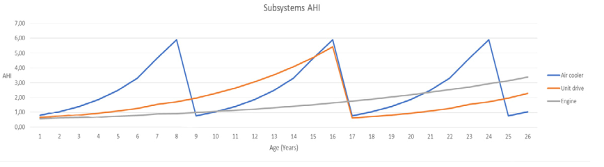
Figure 2. Health index for the different subsystems of an asset.
Interpretation of the value of the Output Index.
The first range is between the values AHI = 0.5 and AHI = 4. The behaviour of the equipment in this range is similar to that of a new equipment.
The second range, which is comprised between the values AHI = 4 and AHI = 6, corresponds to the period of time in which the first symptoms of wear on the equipment begin to appear. In this range, the value corresponding to AHI = 5.5, is the value of the health index equivalent to the normal life expected for the type of equipment under study, as well as each subsystem thereof.
From this period, three intervals are contemplated in the methodology as the AHI index exceeds the values of 6, 7 and 8 respectively.
The methodology assumes that exceeded the value of AHI = 8, the equipment is at the end of its useful life.
The following table (table 1) shows the different ranges of the health index. In this case, it corresponds to an asset with a normal life expected of 50 years, so the remaining life is adjusted to this particular case. On the other hand, the recommendations for action can be applicable to any specific equipment case.
| AHI | Condition | E x p e c t e dLifetime | Requirements |
| 4 – 0.5 | Very good | More than 15 years | Normal maintenance |
| 6 – 4 | Good | More than 10 years | Normal maintenance |
| 7 – 6 | Fair | From 3 – 10 years | Increase diagnostic testing, possible re-placement depending on criticality |
| 8 – 7 | Poor | Less than 3 years | Start planning process to replace |
| 10 – 8 | Very poor | Near to the end oflife | Immediately assess risk; replace or re-build based on assessment |
Table 1. Asset Health index and expected lifetime.
Process pumps fleet application to support maintenance and replacement strategies.
An example of application of the methodology is the case of a fleet of process pumps that are part of the critical systems of a plant. The functional loss of any of these pumps can result in unacceptable situations for the business, such as plant shutdowns, production losses or some type of impact with associated industrial or environmental damage.
In order to establish the appropriate operation scenarios, the plans for major maintenance and equipment substitutions are made based on the health index and not depending on the hours of operation as usual.
In this case, the MS and MF variables that are taken into account for the model are shown in the following table (table 2)
| Measurable Variable | Health modifier))MS | Reliabilty)modifier (MF | Score |
| Vibration analysis | x | 0.5 | |
| Thermal jump between inletand output of the pump | x | 0.5 | |
| Power consumption | x | 0.4 | |
| nº start-up/shutdowns | x | 0.25 | |
| nº of alarms & shots due to lowintake pressure | x | 0.25 | |
| )Speed )rpm | 0.25 | ||
| Fluid leaks | 0.25 | ||
| Oil analysis | 0.2 | ||
| Motor isolation analysis | 0.2 | ||
| Number of corrective mainte-nances | x | 0.2 | |
| Inactivity of the pump | x | 0.15 | |
| Number of overhauls | x | 0.1 |
Table 2. Health & reliability modifiers (MS, MF) for process pumps.
The score obtained for the critical process pumps fleet (figure 3), appears ordered from lowest to highest AHI. Pumps with a lower AHI (H <4), which are in the left area of the graph, have a condition and a failure rate that can be similar to that of a new equipment. On the other hand, pumps with a higher health index (H> 4) begin to behave like more aging equipment in which their failure rates begin to increase and consequently, the associated risk increases from the point of criticality.
The size of each circumference indicates the difference between the initial health index (HIi) and the health index (AHI). Circumferences with larger size indicate that the aging of the equipment has been greater than expected, so it will be necessary to pay more attention to these equipment and increase surveillance. The number that is inside each of the circles indicates the number of overhauls that have been made to the equipment.
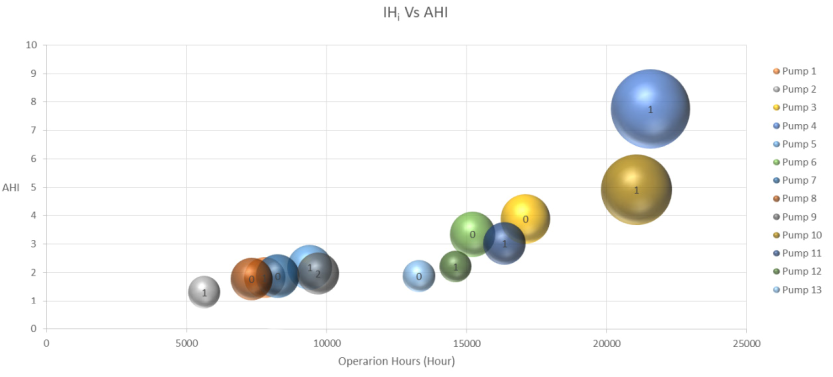
Figure 3. HIi VS AHI for a process pumps Fleet
For those pumps in which the AHI has exceeded 5.5 points, it is necessary to consider major repair or replacement in relatively close periods, including stopping operations until a deep diagnosis has been made to rule out possible problems during its functioning. In the example, pumps 4 and 10 should stop operating and raise the overhaul or replacement. Pump 11 with more hours of operation than pump 6 (17000 vs 15000) has a lower aging (AHI = 3.5 vs AHI = 4.1). This is because the load to which the pump is subjected and the results of the variables of the health modifiers are less aggressive in 11 than in 6. Probably, if the operating and contour conditions do not change, the overhaul of pump 11 will be carried out later (greater than 20000 hours of operation), however, pump 6 will have to be done before the manufacturer’s recommendation.
Conclusions. #
Today, the use of tools for decision making about long-term renewal and replacement of equipment for organizations is quite extended. Thanks to life-cycle cost analysis (LCC), it is possible to know from an economic point of view, the cost of an asset over its useful life and to estimate the time for replacement if needed. The disadvantage in many cases, is the large amount of variables that must be handled when estimating the real cost of an asset over its useful life, generating a scenario of high uncertainty. At that moment, it is where the AHI comes into play as a support tool, having a completely different calculation methodology, estimated from lab tests in order to know the asset condition, visual inspections, operation and maintenance history and the age of the equipment and its components. Using asset health index offers a lot of advantages, such as, provide an approaching indication of the asset at the end of its useful life, prediction of long-term needs replacement in large volumes of assets, identifying potential peaks with investment requirements, identify problems, risks and opportunities for maintenance management, etc.
References #
Abichou, B., A. Voisin, and B. Iung. 2015. “Choquet Integral Capacity Calculus for Health Index Estimation of Multi-Level Industrial Systems.” IMA Journal of Management Mathematics 26(2):205–24.
Abichou, B., A. Voisin, B. Iung, P. Do Van, and N. Kosayyer. 2012. “Choquet Integral Capacities-Based Data Fusion for System Health Monitoring.” IFAC Proceedings Volumes 45(20):31–36.
Azmi, A., J. Jasni, N. Azis, and M. Z. A.Ab. Kadir. 2017. “Evolution of Transformer Health Index in the Form of Mathematical Equation.” Renewable and Sustainable Energy Reviews 76(March):687–700.
Durairaj, Senthil Kumaran, S. K. Ong, A. Y. C. Nee, and R. B. H. Tan. 2002. “Evaluation of Life Cycle Cost Analysis Methodologies.” Corporate Environmental Strategy 9(1):30–39.
Hjartarson, Thor and Shawn Otal. 2006. “Predicting Future Asset Condition Based on Current Health Index and Maintenance Level.” in ESMO 2006 – 2006 IEEE 11th International Conference on Transmission & Distribution Construction, Operation and Live-Line Maintenance.
Ludovic Rizzolo, Bouthaina Abichou, Alexandre Voisin, Naïm Kosayyer. 2011. “Aggregation of Health Assessment Indicators of Industrial Systems.” in The 7th conference of the European Society for Fuzzy Logic and Technology, EUSFLAT-2011.
Naderian, A., S. Cress, R. Piercy, F. Wang, and J. Service. 2008. “An Approach to Determine the Health Index of Power Transformers.” Conference Record of the 2008 IEEE International Symposium on Electrical Insulation (July 2008):192– 96.
Naderian, A., R. Piercy, S. Cress, J. Service, and W. Fan. 2009. “An Approach to Power Transformer Asset Management Using Health Index.” IEEE Electrical Insulation Magazine Vol.25(No.2):2.
Pompili, M. and F. Scatiggio. 2015. “Classification in Iso-Attention Classes of Hv Transformer Fleets.” IEEE Transactions on Dielectrics and Electrical Insulation 22(5):2676–83.
Scatiggio, F., M. Rebolini, Terna Rete Italia, and M. Pompili. 2016. “Health Index: The Last Frontier of TSO’s Asset Management.” 1–9.
Scatiggio, Fabio and Massimo Pompili. 2013. “Health Index : The TERNA ’ S Practical Approach for Transformers Fleet Management.” (June):178–82.
Vermeer, M., J. Wetzer, P. van der Wielen, E. de Haan, and E. de Meulemeester. 2015. “Asset-Management Decision- Support Modeling, Using a Health and Risk Model.” PowerTech, 2015 IEEE Eindhoven 1–6.


