


Maria Psarodimou*, Nikodimos Nikolaidis*, Athanasios Naskos*, George Efremidis*
Atlantis Engineering SA, Greece psarodimou@abe.gr, nikolaidis@abe.gr, naskos@abe.gr, ge@abe.gr
Abstract #
Remaining Useful Life (RUL) estimation is a crucial factor of Predictive Maintenance. Through the predictive maintenance the maintenance departments of the industry field are able to increase the efficiency of the maintenance process, planning well in advance all its aspects. This research work proposes a data-driven RUL estimation approach based on the Long Short-Term Memory (LSTM) algorithm, which is a type of Recurrent Neural Network. LSTM is a supervised method that requires a sizeable amount of run-to-failure historical data, which, in most real industrial environments are hard to obtain as the end-of-life or failure incidents of the critical equipment are rare. To alleviate this issue, we propose a data over-sampling approach to artificially increase the number of run-to-failure-data. In order to enable the RUL estimation approach to output results in the form of remaining Product Cycles (PCs), we also propose an automated PC detection technique based on a motif detection algorithm. For the evaluation of the approach a real industrial scenario is used.
1 Introduction #
The Remaining Useful Life (RUL) analysis can provide valuable information regarding the deterioration rate of assets, as the former is defined as the length from the current time to the end of the useful life. Accurate RUL estimation plays a critical role in the improvement of the quality of the produced products and in the Zero-Defect Manufacturing process in general. Providing accurate estimations of the remaining working hours of a machine or the remaining number of items that the machine can produce (i.e., remaining product cycles), enables the production and maintenance engineers to be well prepared, scheduling in advance the production plan, or obtaining the required parts for maintenance, in order to minimize the downtime of the machine.
RUL estimation can be approached with different techniques, that rely on two main families, the model-based and the data-based techniques. Model-based techniques rely on statistics, like distribution fitting, in order to map the distribution of the actual data to a known distribution and provide the probability of a failure based on a survival function, as it is depicted in the example below (Figure 1).
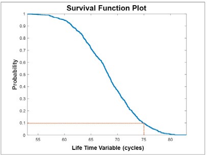
Figure 1: Survival function plot indicating at the end of 75 cycles, the probability of a battery’s continuing to operate is 0.1, or 10%1.
The example of the figure presents the remaining useful life of a battery, showing its deterioration of its life time.
1 source: https://www.mathworks.com/content/dam/mathworks/ebook/estimating-remaining-useful-life-ebook.pdf
Data-driven techniques like similarity models, Figure 2, capture degradation profiles (blue) based on run-to-failure data. The distribution of the asterisks (or endpoints) of the nearest blue curves gives a RUL of 65 cycles for the current data (red).
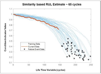
Figure 2: Similarity models capture degradation profiles (blue) based on run-to-failure data. The distribution of the stars (or endpoints) of the nearest blue curves gives a RUL of 65 cycles for the current data (red). Source: mathworks2
More advanced data-driven techniques like the one of this work, propose the use of Neural Networks (NNs) algorithms trained with run-to-failure data in order to estimate the current RUL, either in remaining working hours or product cycles. Properly trained data-driven techniques can outperform the model-based ones, as they are adjusted to specific use cases and do not rely on fixed distributions. However, this type of analysis requires a large amount of run-to-failure data for the training of the network, that in real industrial scenarios are difficult to obtain. To address this issue, the present work proposes an over-sampling technique to increase the number of run-to-failure data generating artificial data based on the real ones.
For the scenario showcased in the experimental evaluation section, the output of RUL estimation is required to be in terms of Product Cycles (PCs), indicating the remaining number of items that the machine can produce until the occurrence of a failure. To be able to output the RUL estimation into PCs, the model needs to be trained in a dataset that is split into PCs. However, the number of PCs at a given time point needs to be extracted for the data itself as it is not provided explicitly. To achieve this task, a pattern recognition mechanism is proposed based on motif detection, which is able not only to compute the number of PCs in each time point, but also to identify the exact point where a PC is started and finished.
To summarize, the contribution of this work is threefold:
- It presents an oversampling technique to increase the number of run-to-failure-data.
- It proposes a pattern recognition mechanism to count and identify the PCs.
- And finally, it applies and evaluates a RUL estimation approach based on NNs.
The remaining of the paper is organized as follows. Section 2 presents an overview of related works from the literature on the fields of RUL estimation and data generation. Sections 3 to 5 present the theoretical background of the techniques that are utilized to implement the proposed solution. Section 6 showcases the integration of the RUL estimation approach into a Predictive Maintenance Platform, while Sections 7 and 8 present the experimental evaluation and conclude the work, respectively.
2 Related Work #
The literature is rich of studies concerning both the RUL estimation and the artificial data generation fields. Plethora of works utilize the LSTM algorithm3, as in the current work, for the RUL estimation due to its performance. Some papers utilize simple LSTM architectures for RUL estimation, such as [4], [5] and [6], where they achieve performance of 85% or score higher than the Support-Vector Machine model accordingly. Specifically in [6], the authors propose the use of a
2 https://www.mathworks.com/content/dam/mathworks/ebook/estimating-remaining-useful-life-ebook.pdf

3 Hochreiter, Sepp, and Jürgen Schmidhuber. "LSTM can solve hard long time lag problems." In Advances in neural information processing systems, pp. 473-479. 1997.
custom feature extraction technique in combination to the LSTM algorithm to enhance its results. Combinations with the LSTM algorithm are popular in the literature. In a variety of papers, the LSTM is combined with other ML techniques for optimization purposes. To mention a few, the authors in [7] utilize a Restricted Boltzmann Machine (RBM) with an LSTM to estimate the RUL and Genetic Algorithms for the model’s parametrization. Their focus rests on the case of partially (under 40%) labelled data. In [8] they develop a deep level LSTM and Convolutional model, which is compared with the model of [9] and is considered satisfactory. The authors of [10] combine a Convolutional and LSTM neural network via a Directed Acyclic Graph to estimate the RUL. [11] proposes Bidirectional LSTMs combined with Linear Regression, while the authors of [12] utilize a Bidirectional Handshaking LSTM with Asymmetric Squared Error as the cost function. Last but not least, [13] uses an LSTM for RUL estimations combined with a mechanism of detecting the cause of error. In our case we propose a simple LSTM model that considers internal motifs (i.e. Product Cycles (PCs)) for optimized results
A common challenge in real applications of RUL estimation, is the lack of a significant amount of properly labelled and suitable data. This can be explained to the transient state of the industry. which is still in the process of familiarizing with the Machine Learning (ML) technologies and their requirements. Thus, it is not uncommon to observe a lack of substantial data or imbalanced datasets that have a great impact on the performance of the supervised ML techniques. For this reason, multiple works focus on the generation of artificial data with various techniques such as Generative Adversarial Networks (GAN) [14]–[16] and DTW, [2] and [17]. [15] utilizes a new variant GAN-based framework called auxiliary classifier GAN (ACGAN) to learn from mechanical sensor signals and generate realistic one-dimensional raw data, while [14] utilizes a Conditional GAN (CGAN) to learn and simulate data. In [16] the authors aim to synthesize ECG signals to prevent the re-identification of individuals, while addressing GAN’s problem of lack of suitable evaluation measures with the introducing of two evaluation metrics specific to their case. Despite their results, GAN networks are also known for training issues such as vanishing gradients, failures to converge and model collapse4. To avoid these issues, we based our data generation mechanism on [2], where the authors utilize DTW’s warping path and a teacher sample for artificial data generation. However, our approach deviates from theirs by utilizing classic DTW and no standard teacher but alternating samples as base samples. Finally, the authors of [17] utilize DTW’s path as a way to combine two different samples.
3 RUL estimation using Neural Networks #
For the RUL estimation, a supervised ML technique is utilized and more specifically a type of Recurrent Neural Networks (RNN) called Long Short-Term Memory neural networks [5].
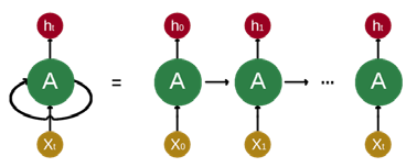
Figure 3: Decomposition of a node in an RNN.
A RNN allows the persistence of information using inner loops. As it is depicted in Figure 3 the output of a node of a RNN in time 𝑡𝑡 is re-fed on the same node along with the input in time𝑡𝑡 + 1. This creates a sequence of recurrent feedings. LSTMs, unlike the traditional RNNs, can efficiently handle the problem of long-term dependencies, which means that for a given timeseries, the problem of recognizing a dependency between points that are far in time, or simply the problem of being able to remember old values along with the new ones. To achieve that, LSTMs maintain a cell state for each neuron and a set of three gates that control the cell state: forget, input, output.
To estimate the RUL of a part of a machine using LSTMs, run-to-failure data are required for the training of the network. Then for each point of time, its preceding n-1 points are considered, creating a sequence of total n-points. n can be quite large since LSTMs can do well at big sequences. These sequences are the training data of the network. Its sequence is mapped to a specific Label (prediction target) which is expressed in the appropriate units (i.e., product cycles, or time units) left till the failure from the last point of the sequence.
The full process for the RUL estimation is presented in Figure 4.
4 https://developers.google.com/machine-learning/gan/gan_structure
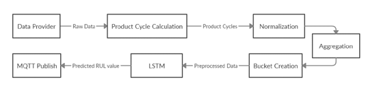
Figure 4: RUL estimation process
The initial step is the data fetching, which is achieved through an implemented service called Data Provider, which communicates with the servers in the shopfloor and fetches the latest sensor measurements to the RUL estimation tool. The data are then forwarded to the component responsible for PC detection that transforms the raw signal to a PC oriented structure. The structured data are pipelined to a transformation process, which includes Normalization, Aggregation and Bucket Creation tasks before being directed to the trained LSTM model for RUL estimation. The result of the tool is circulated back to the plant through a publish in a MQTT broker.
4 Oversampling run-to-failure data #
One of the main requirements of RUL estimation with supervised ML techniques, such as the LSTM algorithm, is the need for a significant amount of data of both normal and faulty behaviour. However, in real industrial environments the required amount of run-to-failure data is not always possible to be obtained since it is an unwanted state that the industries strive to avoid. For this reason, an alternative method for obtaining and increasing the existing amount of data is proposed. More specifically, an artificial data generation technique is implemented that exploits historical run-to-failure data to generate new data with similar characteristics. For the generation of data, the Dynamic Time Warping (DTW) metric [1] is used. The developed technique receives samples of existing faulty data and computes iteratively a user-defined number of similar run-to-failure sequences.
Given two sequences, DTW is used to determine a global distance between them, by matching non-linearly timeseries elements in the time dimension to match features and remove time distortions. To achieve that DTW calculates the minimal path on an element-wise cost matrix using dynamic programming. This minimal path is referred to as the warping path and it provides a mapping of one series to the time steps of another.
The warping path, according to [2], can then be used to produce a warped version of the initial timeseries. This method is called Guided Warping technique and it utilizes the dynamic alignment function of DTW to warp the elements of a reference pattern to the elements of a teacher pattern. The result is a generated pattern that contains features of the input sample at the time steps of the teacher sample.
In our use case, we utilize two distinctive fault instances, and we alternate them as the teacher (base sample). As it is presented in more detail in the next subsection, the information regarding the start and the end of a PC is not provided explicitly, hence it needs to be extracted from the values of a specific measurement that the production engineers had indicated. That means that the artificially generated data need to retain as close as possible the shape of the PCs in order to allow our algorithmic solution to identify the PCs in both the original and the generated data.
The following two figures present a PC from the original data (Figure 5), which is a recurrent motif that signifies that a new product is being processed in the machine and a PC from the generated data (Figure 6), which although it does not maintain the exact shape it maintains some characteristics especially at the beginning and the end of the PC, which allow the PC detection algorithm to work properly.
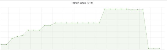
Figure 5: The original data Product Cycle. This motif reappears throughout the dataset and depicts the processing of a new product.
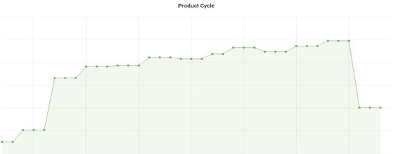
Figure 6: A Product Cycle as observed in a newly generated dataset.
In the figures above we have removed the axes with the magnitute and the time respectively, along with the description of the ploted measurement for confidentiality purposes.
5 Product cycles detection #
In order to estimate the RUL in terms of remaining PCs, it is important to implement a reliable mechanism for PC identification. In the original dataset, we have used a condition-based mechanism to identify the PCs in the raw signal, however the generated data present slight alternations both from the original data and the different generated sequences, so use of the condition-based approach is not possible.
For this reason, we have implemented a more reliable PC detection technique, which is based on a similarity search algorithm. The Mueen’s Algorithm for Similarity Search (MASS)6 algorithm [3], calculates the Distance Profile (DP) of a query with a timeseries in an efficient way. A DP is a vector of the Euclidean distances between a given query and each subsequence in a timeseries. The sub-sequences are obtained by sliding a window of length m or the length of the query. The MASS algorithm computes the DP with a complexity of O(nlogn) by exploiting the fast Fourier Transform (FFT) algorithm to calculate the dot products between the query and all sub-sequences of the time series as, depicted on Figure 7.

Figure 7: An example of convolution operation for the sliding product and consequently the Distance Profile calculation.
6 https://www.cs.unm.edu/~mueen/FastestSimilaritySearch.html
In our implementation, we calculate the DP of a historical sample of a single PC with the fully generated dataset, locating the start of a potential match and thus the beginning of a new PC. In the example of Figure 8 we provide the first motif as the representative sample and detect the following ones that are depicted with the red line.
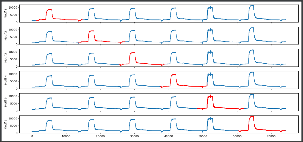
Figure 8: A MASS based PC detection example that utilizes the first motif as a historical profile and detects the upcoming ones. The detected motifs are depicted with the red lines.
In this paper we utilized the PC depicted on Figure 9 as the representative sample. The PCs are detected with a distance threshold that can be defined by the user. This distance threshold controls the amount of the detected PCs based on their similarity level. The higher the distance threshold the more PCs are detected due to lower similarity constraint. For example, setting the distance threshold to 4, as depicted in the upper plot of Figure 10, detects more PCs (red dots) than the other two cases (i.e., middle and bottom plots) with distance thresholds 3.5 (blue dots) and 3 (orange dots), respectively.

Figure 9: The PC that we utilized as a historical sample for PC detection.
OM

Figure 10: The detected PCs for different distance threshold. The red dots depict PCs with a distance threshold of 4, the blue dots PCs of distance threshold 3.5 and the yellow PCs with distance threshold of 3.
6 Integration to predictive maintenance platform #
The proposed algorithms are encapsulated to a predictive maintenance platform, which allows the maintenance engineering to configure and instantiate the RUL estimation process and monitor its results through a visualization dashboard. The platform implementation is based on a micro-services architecture. The user interface is implemented on the angular framework and the micro-services can operate either through the web interface or through the provided API endpoints.
The platform offers forms for parametrization of the various micro-services, a Task’ status page, a KPI’s page as well as integrated visualization dashboards to enable easy data and results monitoring. The following figures, Figure 11 and Figure 12, depict two pages that fetch data and initialize a RUL estimation model accordingly.

Figure 11 Smart maintenance platform form for data fetching configuration.
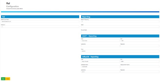
Figure 12 Smart maintenance platform form RUL estimation process configuration
7 Experimental Evaluation #
7.1 Training – Testing Dataset formation #
Our experimentation focuses on the RUL estimation of a specific component of a grinding machine from a big grinding and lather machines manufacturer. The goal is to provide accurate RUL estimation to this critical part of the machine, to achieve Zero-Defect Manufacturing and to satisfy customer quality requirements by systematizing quality control. The selected part, which is presented in Figure 13, is a grinding wheel with high productivity and constant working conditions, which has a higher probability of failure than the other components, hence its close monitoring is crucial. Deviations or variability in the working conditions of the machine, might be an indication of high deterioration of the machine condition, that could affect the grinding process and cause geometry or quality defects, which in turn, cause the need for extensive rework and increase of the produced scrap.
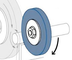
Figure 13: Grinding wheel used for the RUL estimation analysis.
The provided dataset spans across 11 months of constant production, where there are only two occurrences of failure into the specific component, thus the dataset is highly unbalanced with an influx of normal behaviour data and only scarce appearances of faulty behaviour data.
To compensate this behaviour, we applied our data generation technique to oversample the run-to-failure data. For this purpose, we utilized two sets of 12-hour data close to each reported failure and generated similar datasets that mimic the behavior of the grinding machine when it is close to the reported failures. Through this process we have created 5 added run-to-failure datasets.
Next, followed the detection of the PCs using the implemented technique based on the MASS algorithm, setting a distance threshold to 3 in order to detect as similar PCs as possible. The distance threshold was set after an iterative experimentation process with different parametrizations. After some steps of pre-processing that transform the generated data to compatible formats, the training and testing sets were ready to be forwarded to the RUL estimation tool with the LSTM algorithm for evaluation.
The architecture of the utilized NN is a double layered LSTM model, where the first layer contains 100 units followed by 20% dropout rate and a second layer of 50 units and 20% dropout rate. The last network layer is a dense output layer of a single unit. The model uses a linear activation function, the mean squared error metric for the loss function and the mean absolute error metric for the LSTM’s performance.
Once trained the model is loaded in a TensorFlow server (TFX). A TFX is a Google-production-scale machine learning platform, based on TensorFlow. It provides a configuration framework and shared libraries to integrate common components, needed to define, launch, and monitor a machine learning system.
7.2 Experimental Results #
The presented experimental results of this section are derived through a cross-validation process, where the 5 run-to- failure datasets are split into 4 datasets for training and 1 for testing, producing all the 5 different combinations.
Table 1: Mean Absolute Error results derived through the cross-validation process.
| 1st iter. | 2nd iter. | 3rd iter. | 4th iter. | 5th iter. | Average | Std. | |
| MAE | 59.92 | 67.8 | 42.76 | 81.67 | 82.91 | 67 | 14.8 |
As it is depicted in the Table the average Mean Absolute Error (MAE) is 67. Since the estimation is between 1 and 300 Product Cycles that means that our estimation is off by +-22%. However, as we observe in Figure 14 and Figure 15 as the machine approaches the end of life the estimation becomes more accurate.

Figure 14 : RUL estimation result achieved on the 1st iteration of the cross-validation process. The green line indicates the actual value while the blue the estimated one.
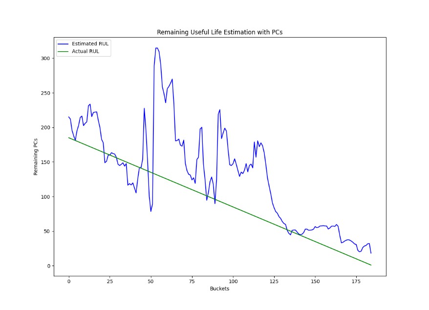
Figure 15 : RUL estimation result achieved on the 3rd iteration of the cross-validation process. The green line indicates the actual value while the blue the estimated one.
8 Conclusions #
RUL estimation assists the maintenance departments to increase the efficiency of the planned maintenance process decreasing the downtime of the machines, by planning all the aspects of the maintenance well in advance. This work proposes a RUL estimation technique based on the LSTM algorithm, in combination with a data generation approach in order to over-sample the run-to-failure data, needed for the accurate training of the model. In order to provide results in the form of remaining PCs, an automated approach of PC detection is implemented based on the MASS algorithm.
The presented algorithmic solution was encapsulated into a predictive maintenance platform, offering a user-friendly graphical interface to the maintenance engineers in order to instantiate and monitor the RUL estimation process.
For the evaluation of the proposed approach, data from a real industrial environment are used and more specifically from a grinding machine. The results obtained from a 5-fold cross validation process, indicate that the model is able to learn the RUL based on the provided artificially generated data, especially when the machine approaches its end of life.
As a future work, as the production continues, the occurrence of more failure incidents will assist the generation of more accurate artificial data and RUL estimation models.
9 References #
- T. Giorgino, “Computing and visualizing dynamic time warping alignments in R: The dtw package,” J. Stat. Softw., vol. 31, no. 7, pp. 1–24, 2009, doi: 10.18637/jss.v031.i07.
- B. K. Iwana and S. Uchida, “Time series data augmentation for neural networks by time warping with a discriminative teacher,” Proc. – Int. Conf. Pattern Recognit., pp. 3558–3565, 2020, doi: 10.1109/ICPR48806.2021.9412812.
- C. C. M. Yeh et al., “Time series joins, motifs, discords and shapelets: a unifying view that exploits the matrix profile,” Data Min. Knowl. Discov., vol. 32, no. 1, pp. 83–123, Jan. 2018, doi: 10.1007/s10618-017-0519-9.
- O. Aydin and S. Guldamlasioglu, “Using LSTM networks to predict engine condition on large scale data processing framework,” in 2017 4th International Conference on Electrical and Electronics Engineering, ICEEE 2017, May 2017, pp. 281–285, doi: 10.1109/ICEEE2.2017.7935834.
- H. Wu, A. Huang, and J. W. Sutherland, “Avoiding Environmental Consequences of Equipment Failure via an LSTM-Based Model for Predictive Maintenance,” Procedia Manuf., vol. 43, pp. 666–673, 2020, doi: 10.1016/j.promfg.2020.02.131.
- Y. Wu, M. Yuan, S. Dong, L. Lin, and Y. Liu, “Remaining useful life estimation of engineered systems using vanilla LSTM neural networks,” Neurocomputing, vol. 275, pp. 167–179, Jan. 2018, doi: 10.1016/j.neucom.2017.05.063.
- A. Listou Ellefsen, E. Bjørlykhaug, V. Æsøy, S. Ushakov, and H. Zhang, “Remaining useful life predictions for turbofan engine degradation using semi-supervised deep architecture,” Reliab. Eng. Syst. Saf., vol. 183, pp. 240– 251, Mar. 2019, doi: 10.1016/j.ress.2018.11.027.
- A. Z. Hinchi and M. Tkiouat, “Rolling element bearing remaining useful life estimation based on a convolutional long-short-Term memory network,” in Procedia Computer Science, 2018, vol. 127, pp. 123–132, doi: 10.1016/j.procs.2018.01.106.
- E. Sutrisno, H. Oh, A. Vasan, and M. Pecht, Estimation of remaining useful life of ball bearings using data driven methodologies. 2012.
- J. Li, X. Li, and D. He, “A Directed Acyclic Graph Network Combined With CNN and LSTM for Remaining Useful Life Prediction,” IEEE Access, vol. 7, pp. 75464–75475, 2019, doi: 10.1109/ACCESS.2019.2919566.
- C. G. Huang, H. Z. Huang, and Y. F. Li, “A Bidirectional LSTM Prognostics Method Under Multiple Operational Conditions,” IEEE Trans. Ind. Electron., vol. 66, no. 11, pp. 8792–8802, Nov. 2019, doi: 10.1109/TIE.2019.2891463.
- A. Elsheikh, S. Yacout, and M. S. Ouali, “Bidirectional handshaking LSTM for remaining useful life prediction,” Neurocomputing, vol. 323, pp. 148–156, Jan. 2019, doi: 10.1016/j.neucom.2018.09.076.
- M. Yuan, Y. Wu, and L. Lin, Fault diagnosis and remaining useful life estimation of aero engine using LSTM neural network. 2016.
- R. Fu, J. Chen, S. Zeng, Y. Zhuang, and A. Sudjianto, “Time Series Simulation by Conditional Generative Adversarial Net,” Int. J. Neural Networks Adv. Appl., vol. 7, pp. 1–33, 2020, doi: 10.46300/91016.2020.7.4.
- S. Shao, P. Wang, and R. Yan, “Generative adversarial networks for data augmentation in machine fault diagnosis,” Comput. Ind., vol. 106, pp. 85–93, 2019, doi: 10.1016/j.compind.2019.01.001.
- A. M. Delaney, E. Brophy, and T. E. Ward, “Synthesis of Realistic ECG using Generative Adversarial Networks,” pp. 1–16, 2019, [Online]. Available: http://arxiv.org/abs/1909.09150.
- M. Akyash, H. Mohammadzade, and H. Behroozi, “DTW-Merge: A Novel Data Augmentation Technique for Time Series Classification,” pp. 1–6, 2021, [Online]. Available: http://arxiv.org/abs/2103.01119.


